Benchmarking BiocRefgetStore vs BSgenome/Biostrings

BiocRefgetStore exposes a BSgenome-compatible interface to sequences backed by a RefgetStore (via the Rust-backed gtars crate). This vignette compares sequence extraction with the RefgetStore backend in this package (RefgetGenome) against the classic Bioconductor stack (BSgenome::getSeq() on a real BSgenome object).

The numbers below are reference measurements committed to the package, taken on one maintainer machine on the full human genome (GRCh38/hg38) -- the 25 primary chromosomes of BSgenome.Hsapiens.UCSC.hg38, with the RefgetStore built from that same assembly so the comparison is exact. Treat the absolute times as illustrative -- they depend on the hardware that produced them -- and read the table for the shape of the comparison: which backend wins which kind of access, and by roughly how much. The measurements are reproducible from the package's own harness (run_benchmarks(), defined in R/benchmark.R); see the comment at the top of this file to regenerate them.

The two backends

RefgetGenome (this package). Built from a FASTA, a directory store, or a remote refget store. Sequences are addressed by digest, and the bulk extraction path (extractRegions()) hands an entire region set to Rust in a single foreign-function call, so per-region R overhead does not accumulate. See Getting Started for construction details.

BSgenome (the comparator). The long-standing Bioconductor representation of a genome. BSgenome::getSeq() reads from an on-disk 2bit blob memory-mapped into the session. Whole-chromosome and in-memory access are its sweet spot.

To make the comparison apples-to-apples, the committed run builds the RefgetStore from a FASTA exported from BSgenome.Hsapiens.UCSC.hg38 itself, and benchmarks against that same installed BSgenome data package. Both backends therefore see identical seqnames and coordinates, and the harness asserts that the extracted sequences match (the Match column below). An indexed-FASTA Rsamtools::FaFile is included as a secondary baseline. (When no BSgenome package is supplied, the harness instead forges a real in-memory BSgenome from the FASTA, which is how it runs on the small bundled genome with no data-package install.)

The harness

The whole comparison is one call. run_benchmarks() builds the contestants from a FASTA, warms each one (so index loads and mmap faults are excluded from timing), times single-region, bulk multi-region, and full-chromosome extraction, and returns a tidy data frame with one row per (operation, backend): operation (single / bulk / full_chrom), backend, n_regions, total_bp, median_time (seconds), mem_alloc, iterations, and check (did this backend's output match the reference?).

The refget backend appears as two rows, to separate extraction from formatting:

• refget_converted returns a Biostrings DNAStringSet/DNAString, the same object type bsgenome and fafile produce. This is the apples-to-apples comparison.
• refget_raw returns the plain character vector that gtars hands back, with no DNAStringSet ever constructed (getSeq(..., as.character = TRUE)).

The two differ only by the Biostrings conversion, so the gap between them is exactly what that conversion costs. The interesting result: a large share of refget's reported time is that conversion (the majority of it for whole-chromosome extraction) -- and even so, refget wins every operation.

Timing results

Median time in milliseconds, throughput in megabases per second, and the cross-backend correctness flag (bulk here is 2000 regions).

results <- readRDS(res_file)
tab <- results
tab$median_ms <- round(tab$median_time * 1e3, 3)
tab$mb_per_s <- round((tab$total_bp / 1e6) / tab$median_time, 1)
tab <- tab[order(tab$operation, tab$median_time),
           c("operation", "backend", "n_regions", "total_bp",
             "median_ms", "mb_per_s", "check")]

knitr::kable(
  tab,
  col.names = c("Operation", "Backend", "N regions", "Total bp",
                "Median (ms)", "MB/s", "Match"),
  row.names = FALSE,
  caption = "Median extraction time by operation and backend (lower is faster)."
)

Table: Median extraction time by operation and backend (lower is faster).

Operation	Backend	N regions	Total bp	Median (ms)	MB/s	Match
bulk	refget_raw	2000	2000000	23.764	84.2	TRUE
bulk	refget_converted	2000	2000000	32.488	61.6	TRUE
bulk	fafile	2000	2000000	51.906	38.5	TRUE
bulk	bsgenome	2000	2000000	390.524	5.1	TRUE
full_chrom	refget_raw	1	248956422	722.490	344.6	TRUE
full_chrom	refget_converted	1	248956422	1733.175	143.6	TRUE
full_chrom	fafile	1	248956422	1881.384	132.3	TRUE
full_chrom	bsgenome	1	248956422	4296.931	57.9	TRUE
single	refget_raw	1	1000	0.217	4.6	TRUE
single	refget_converted	1	1000	0.388	2.6	TRUE
single	fafile	1	1000	5.058	0.2	TRUE
single	bsgenome	1	1000	41.028	0.0	TRUE

Comparison plot

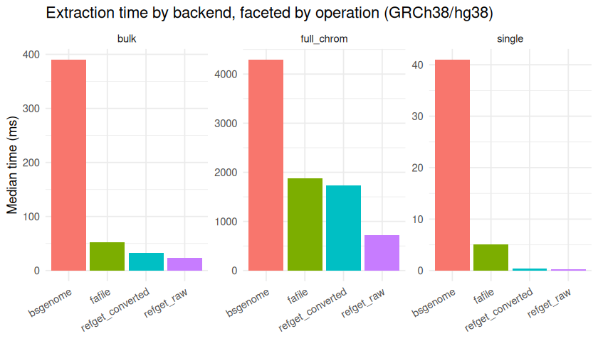
plot of chunk plot

How to read this

On this genome, the RefgetStore backend is the fastest in every operation -- single-region, bulk multi-region, and whole-chromosome -- ahead of both BSgenome::getSeq() and the indexed-FASTA FaFile baseline, with all backends returning identical sequence (the Match column). The size of the margin, and where it comes from, varies by operation:

• Bulk multi-region extraction (bulk) is the standout. extractRegions() passes the whole region set across the FFI boundary in a single in-memory call (no temp file, no per-region R object boxing), so the per-region R-level overhead that grows with the region count never accumulates. This is the workload to watch in the table above. Compare refget_raw against refget_converted here: the raw character path is markedly faster, so a large share of the converted row's time (≈27% on this run) is the Biostrings DNAStringSet construction, not the store read -- and even with that conversion, refget_converted still wins. If you only need a character vector, the raw path is dramatically faster.
• Full-chromosome extraction (full_chrom) returns one whole contiguous sequence. The raw-vs-converted gap is even larger here -- roughly 58% of the converted time is the DNAStringSet construction rather than decoding the store -- yet refget_converted is still ahead of BSgenome and the FaFile baseline.
• Single-region extraction (single) is dominated by fixed per-call overhead in every backend, so the times are tiny and the absolute differences are small; don't over-read them.

There is also a one-time setup cost that the harness deliberately excludes from timing: constructing the RefgetGenome store, indexing the FASTA, or forging/loading the BSgenome. If you only ever read one region, that setup cost dominates everything in the table. And as noted above, treat the absolute times as illustrative -- they are hardware-dependent, so read the table for shape and magnitude rather than exact milliseconds.

See the Reference vignette for the complete API.

Regenerating

The committed results come from the maintainer script data-raw/benchmark.R, which exports the GRCh38 primary chromosomes from BSgenome.Hsapiens.UCSC.hg38 to a FASTA, builds a RefgetStore from it, runs run_benchmarks(), and writes the committed vignettes/benchmark_results.rds + vignettes/benchmark_plot.png. It needs the benchmark Suggests (bench, BSgenome, rtracklayer, Biostrings, ggplot2) plus the hg38 data package installed, and a few GB of scratch disk:

Rscript data-raw/benchmark.R

To benchmark a different assembly, name another installed BSgenome data package and a matching FASTA -- or call the harness directly:

res <- run_benchmarks(
  fasta_path   = "sacCer3.fa",                        # FASTA of that assembly
  bsgenome_pkg = "BSgenome.Scerevisiae.UCSC.sacCer3",
  n_bulk       = 2000
)
knitr::kable(res)